AGE AND GROWTH OF THE DAB, Limanda limanda (LINNAEUS) IN ISLE OF MAN WATERS, UK

Trabajo recibido el 4 de septiembre de 1985 y aceptado para su publicación el 15 de febrero de 1988.

RESUMEN

INTRODUCCIÓN

It is well know, through the literature on fish, that growth (within the limits of the species) mainly depends, on the availability of food, which in turn could be subject to productivity of the area and/or density of population. It is possible that denser population or lower productivity means greater competition for available food, therefore over populated areas or areas with low productivity may have low rates of growth. This assumption gives a basis for calculating the rate of growth of dab and it could provide an index of productivity, density and to some extent fishing effects in the area.

There was no specific data available on productivity, density and fishing effects related to dab population in the area but length and weigth data at age was available. It is proposed that characteristics of the growth curve might be the result of availability of food in the area. Nikol'skii (1961) shows several examples of different growth curves for the same species in different areas.

The aims of this study are as follows:

1. Find an appropiate growth model for dab.

2. Relate growth to seasonal conditions in an attempt to predict what effect fluctuations in seasonal conditions have on growth.

3. Use the overall weight-length relationship and gutted weight-length relationship to calculated weight and gutted weight at age, respectively.

4. Show the weight differences between the whole weight and gutted weight for a given length at age.

5. Estimate natural mortality using the rate of decrease in growth (K).

Dab were caught around the coast of the Isle of Man between 54° 00' and 54° 25' N, 4° 55' and 4° 10' W in depths from 4 to 40 m. A few additional samples were taken 20 miles E of the Isle of Man at a depth of 20 - 40 m, and 3 miles SE of the Isle of Man between 30 - 50 m. Monthly samples were taken, weather permitting, from November 1976 to March 1979 by means of an otter trawl with wings of 70 mm mesh size and cod end of 45 mm. Weekly samples of young fish were taken in Port Erin Bay at depths of 4 - 8 m (whenever possible) from April 1977 to May 1979, using a beam trawl with mesh size of 60 mm, exterior net, and 15 mm interior lining net. A total of 4,340 dabs were examined.

Dab which were not processed within 24 hrs of captured were frozen for up to three or four weeks. Trawled fish were measured to the nearest mm and weighted to the nearest g. The otoliths were easy to read. Age at capture was reduced from the number of opaque (summer) bands an hyaline (winter) rings on the otolith. It was assumed that all dab had hatched in May and the age was recorded in months (Ortega, 1981a; 1981b).

Records of each fish were maintained as computer file. The results were processed in the ICL 1906A computer from the University of Liverpool and the CDC 7600 from the University of Manchester using the Statistical Package for the Social Sciences, version 5 and 6, respectively. Scattergrams represented individual data points by means of an asterisk (*). More than one asterisk in the same position was marked by a figure (1-9) to indicate the number of fish, however all the data were used for the calculations. Scales differed on a given pair of scattergrams for males and females, because a feature of the computer program was an automatic scale for the data provided. Lines showing range of values were fitted by eye. The symbol (x) represented one specimen: and (o) indicated that 0.95 C.I. were too big to plot.

We shall try to use the rate of growth of the population of dab sampled around the Isle of Man, whose geographical position may be considered here as an index of the Irish Sea. The NE part of the Irish Sea has been sampled for sole and plaice since 1975, in order to predict future catches and obtain information on demersal species such as dab in the Irish Sea (Leeuween, 1975-1978).

Ageing the dab was relatively easy (Ortega-Salas, 1980,1981a, 1981b). The number of female and male fish caught by otter and beam trawl at each age-gp is shown in the Table 1.

Many of the 0-gp and early 1-gp fish were taken in Port Erin Bay by beam trawl. Offshore most of the dab were caught by otter trawl. They were between 1 and 4 years old. The 45 mm cod end mesh of the otter trawl selects against very young fish. Male dab older than 4 years, were less common than female dab of the same age. Dab over 6 years were rearely caught. There was wide range of length for age in both sexes (Fig. 1). It was seen that larger dab at a given age were not equally represented throughout the year: larger dab disappeared from the samples shortly before spawning time in April-May.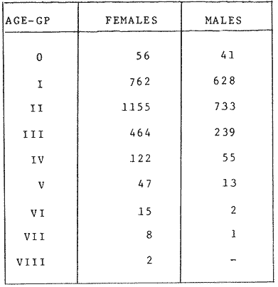

TABLE 1 THE NUMER OF FEMALE FISH CAUGHT BY OTTER AND BEAM AT EACH AGE-GP

A routine computer program was used to show the behaviour of the population sampled in a two-dimensional space. The programme also calculated the straight regression line length at age but a curvilinear relationship described the data better as is usual in the analysis of fish. This became clear when mean length for age was plotted at two monthyly intervals, as shown in figure 2. It may be interpreted from these figures that growth from June-November is related to a clear group of fish, which seems to be different from the group in December-May, possibly because bigger fish at each age have emigrated of died. It would seem however, that dabs grew most rapidly in summer (June-October) (environmental conditions in summer and better than winter), and that females grew faster than males after year 2.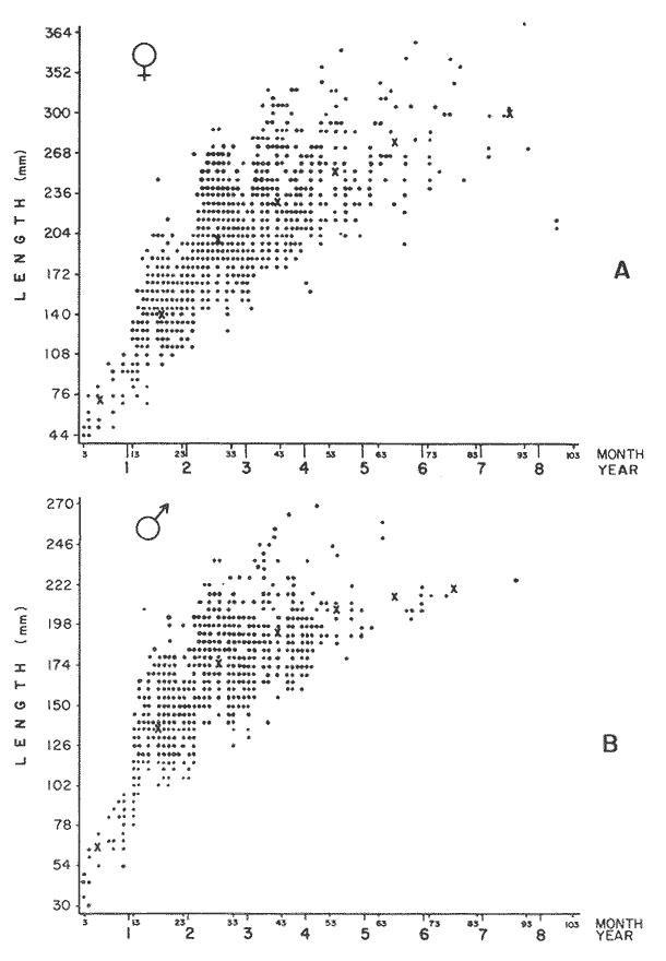

Figure 1. Total fish length for age at monthly intervals. Calculated mean length id represented by (x). A= females; B = males.

A von Bertaleffy's curve (von Bertalanffy, 1951) is often considered appropiate to describe growth in length or weight at age (e.g. Beverton and Holt, 1957).

The equation to the curve may be written in the form:

L_t=L∞(1-e^-K(t-to))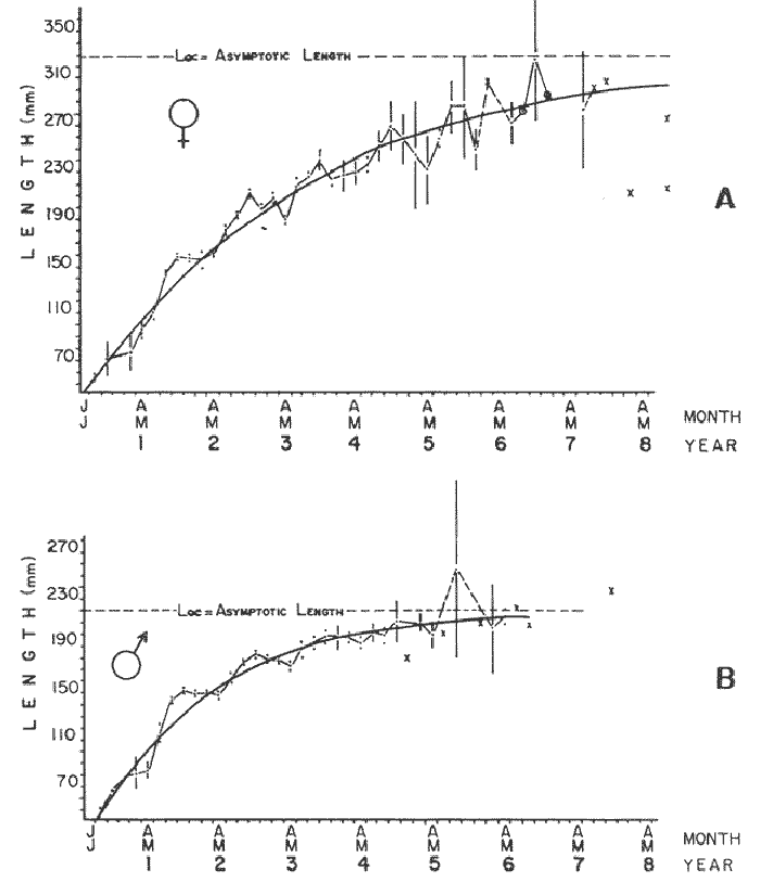

Figure 2. Mean length for age at two monthly intervals with 0.95 C.I. and von Bertalanffy theoretical curve. A= females: L* = 329.73, K = 0.317893, to = 0.239399; B = males: Loo = 221.52, K = 0.6040239 to = 0.42541.

where Lt: length at time (t); Loo: asymptotic or maximum length; K: Constant relating to rate of decline in growth towards reach maximum length; to: time at which the organism would theoretically have zero length; e: base of natural logs (ln).

A computer program in Standard Basic, was written to calculated the parameters of the curve by Holt's method (Gulland, 1969) (see Appendix). A linear regression equation was fitted to the difference in length between time t and t + 1 against mean of the lengths at time to and t + 1 (i.e. Lt + 1 - Lt against ((Lt + 1 + Lt)/2) to determine K (as the slope of the regression and L∞ as the intercept on "X" axis), to was obtained by using observed values of length for age in the von Bertalanffy's equation with the calculated values of K and Loo and solving for to (i.e. to = t + (1/K) ln(L∞(Lt)/L∞).

The lengths at age used in the regression were mean lengths at each age-gp, in years. Calculated from the mean values at 2 months intervals of age-gp (i.e. t was in units of 12 months). The program was initiated with pooled data for 0-gp fish from August and September to April and May. The designate t: 1 corresponded to a fish 3 months old to 12 months, t: 2 to fish 13 months old (June) to 24 months (May), and so on. This smoothing technique consists of stabilizing the lengths at age.

The parameters of the equation solved were the following:

FEMALES: L∞= 329.73. K = 0.317893, to = 0.23939

MALES: L∞= 221.52, k = 0.606023, to = 0.42541

The theoretical curve is shown, with observed mean lengths in figure 2. Despite the seasonal variation, the curve shows a good fit to the observed mean lengths, to is positive and according to the initial interval fits very well to be length almost 0.

Fabens, (1965) devised a computer program which used individual values of the growth parameters, to fit the von Bertalanffy growth curves to any set of recapture or agesize data. The parameters of the equation in Fabens' symbols are the following:

X = A (1-Be^-Kt)

where: X: linear size of time (t) = Lt (above); A: asymptotic length= L∞ (above); K: constant rate of growth = K (above); B: A constant related to the size of the animal at birth.

The parameter K and A are calculated by iterated least squares method from data on successive sizes of an animal and the time interval between measurements. The parameter B as calculated by the same method when more than one datum was given. This data consisted of the size of the animal and the respective age giving a (set of) point(s) in the graph through which the curve should pass.

All the individual data for males and females separetely, were used in Fabens' with the following results after 7 interations:

FEMALES: A = 279.5, K = 0.04217, B = 0.9916, n = 2629

MALES: A= 204.8, K = 0.0685 1, B = 0.9957, n = 1711

The computed lengths at age were plotted as a growth curve, however when the resulting curve was fitted to the mean length at each age it was not considered to be good (Fig. 3) (by eye). The mass of data at ages 1 to 3 years produced a heavy weighting at those ages, consequently younger and older fish had comparatively little effect on the parameters of the equation. Fabens' curve fits the centre of gravity of the data points.

Fabens' equation was then recalculated using the values mean length at each age-gp (from the mesh values at each two months interval) as was done for Holt's method" giving the following results after 20 interations:

FEMALES: A = 309.4, K = 0.03369, B = 0.9533, n = 7.

The difference was for

A= 0.0006 and for K = -0.001.

MALES: A = 198.6, K = 1.325, B = 1758, n = 6.

The difference was for A = -0.5 x 10¹⁰ and for K = 0.04. The parameters solved for females gave better results however the results for males were negative for X when solved because B coefficient was too big.

Computed values of length for age by Holt's method (von Betalanffy's) and those of Fabens' program are shown in the Table 2.

The observed mean lengths given in the table serve to illustrate that the new program provided a better fit (judging by eye) to the data than Fabens' program when all the individual data were used. On the other hand, Fabens' results were quite similar, at least for females, to those of von Bertalanffy's when mean length at each age-gp were used.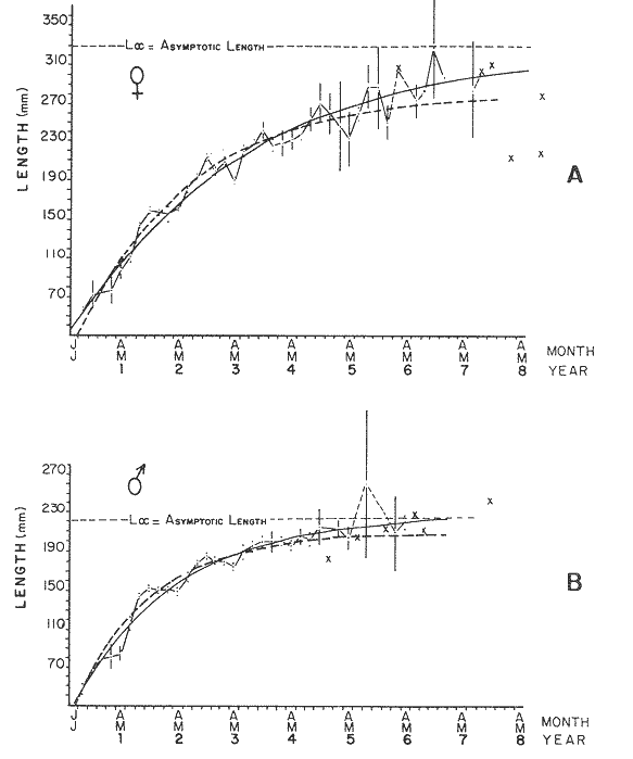

Figure 3. Mean length for age at two monthly intervals with 0.95 C.I. Comparison between von Bertalanffy's (continous curve) and Faben's method (dashed curve). Faben's parameters are: A) females: A = 279.5, K = 0.04217, B = 0.9916, n = 2,629; B) males: A = 204.8, K = 0.06851, B = 0.9957, n = 1,711.

The data have been analysed by the mean length at each age-gp using Holt's method and all the individuals by their length (mm) at age (months) using Fabens' program. Now, we shall try to use Gompertz' growth curve equation analysed which has been widely used in biology (Parrack, 1979; Weymouth et al. 1931) in order to compare the fitting growth calculated points to this data. The equation may be written as follows:

Lt = e^B-Ce^-Kt

Where: Lt: length at time (t) = x (as above); k: constant of rate of growth = K (as above); C: constant (A/k where A: e^a); B: constant (ln L + Ce^-kt where L: observed length; e: exponential form of logs (ln).

Weymouth et al. (1931) described the mathematical derivation to use Gompertz' equation (1825) with the Razor clam (Silique patula) observed length at age. Ln difference between ln lengths at successive increasing ages plotted against the age + 0.5 i.e. Table 3. Gave a negative straight line whose slope is equal to k (t). The equation of that straight line is y = Y + b (x-x), which may be expressed as y = a - b x, where-b is the slope (k), A: e^a, C = A/k. B = LNL + Ce^-kt, where lnL is the natural log of the observed length. The devised program in Standard Basic (with an example) is in the Appendix.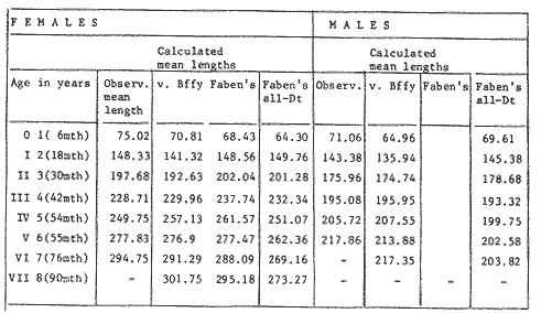

TABLE 2 COMPUTED VALUES OF LENGTH FOR AGE BY HOLT'S METHOD (von BERTALANFFY'S) AND THOSE OF FAVEN'S PROGRAM.

TABLE 3 WEYMOUTH ET AL. (1931) DESCRIBED THE MATHEMATI CAL DERIVATION TO USE GOMPERTZ' EQUATION (1825) WITH THE RAZOR CLAM (Siliqua patula)

The results from Gompertz' equation give the following parameters.

FEMALES: K = 0.44871, B = 5.78042, C = 2.12526, n = 6

MALES: K = 0.63594, B = 5.42439, C = 1.96861, n = 5

The calculated length from Gompertz' equation compared with those of Holt's method and Fabens' program are as follows: Table 4.

Although it is a matter of interpretation, the Table above implies that Holt's method (von Bertalanffy's) gave a better approach to the observed mean length at age-gp, and also compared with the representation of individual fish in the scattergram (Fig. 1) (mainly females) where the population sampled is represented.

Therefore the results from von Bertalanffy's growth model in Isle of Man waters which were taken as an index of the Irish Sea in 1977, would give the basis for comparison with growth results in other areas as a result of the interaction parameters of the ecosystem such as temperature, food available and density which may be related to fishing effects, and others.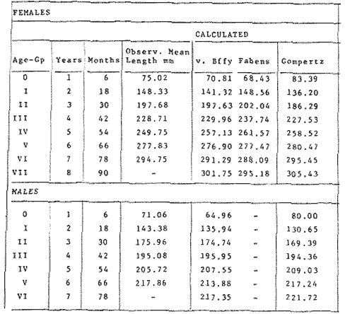

TABLE 4 THE CALCULATED LENGTH FROM GOMPERTZ' EQUATION COMPARED WITH THOSE OF HOLT'S METHOD AND FABEN'S PROGRAM.

It has been suggested that the mean length at age is biased, partly because the bigger fish at each age were absent (either emigrate or died) from the samples and partly because the fish grew faster in summer than winter. Figure 2 shows that October/November is the period when dab reach peak growth and most of the fish are believed to be in the sampled area. The lowest lengths were observed in February/March or April/May, so the data were reorganized for the period of faster, and lowest rates of growth using Holt's method (von Bertalanffy') and Gompertz' equation. The results are shown in Table 5.

The above results showed that, in general the fastest growth period (summer) had a lower value of K, but higher asymptotic length (Lα), therefore higher rate of growth. In winter there was a lower rate of growth, so the asymptotic length was low and K was high. K gives the rate of declining growth; which Lα gives the actual rate of growth.

If we make an analogy of wintering conditions either to summer or to an area of poor conditions and summering conditions (either to winter or to an area of favourable conditions) for a given population it may be that if Lα is high in an area of favourable conditions.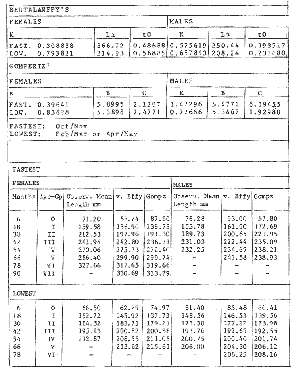

TABLE 5 PERIODS OF FASTEST AND LOWEST RATES OF GROWTH USING HOLTS METHOD (von BERTA LANFFY'S) AND GOMPERTZ' EQUATION.

In another area, of poor conditions. Lα would be smaller, but no necessarily for K which could be inverse. All there would depend on the shape of the growth curve (i) if Lα is high K may be low, and (2) if Lα is low K may be high: figure 4.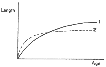

Figure 4. Shape of the growth curve (1) if Loo is high K may be low, and (2) if Loo is low K may be high.

The results show the average limits of the rate of growth as it is at present calculated for dab. A comparison with similar analyses in the area, in future years, may be a useful index since the environmental conditions (according to Brander, 1980) in the Irish Sea are being subjected to great environmental change caused by interference with the ecosystem by such activities as overfishing and pollution.

It could be supposed that the differences in the actual rate of growth or dab might be related to fishing rate, as this could affect densities and consequently would be reflected in changed food availability. Although these results cannot be compared with data from previous years, since there has been no parallel work done in the area, a comparison may be made using the same species in other regions Jonsson (1966) (Fig. 5).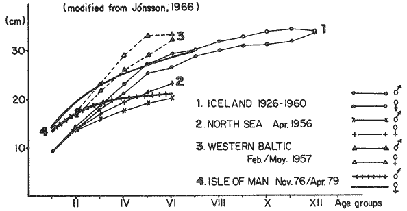

Figure 5. Rate of growth Comparison between dabs from different regions (modified from Jonsson 1966).

This figure suggest that the Icelandic dab has a growth curve whose characteristics are very different from the other areas; for instance, older ages of Icelandic dab could indicate that the total mortality is much lower. In the other areas it is similar. Although the same species the habitat is so different that the Icelandic dab appear to be almost a different species.

Therefore it should no be used to make comparisons in terms of their exploitation. However, using the same figure the rate of growth was calculated using von Bertalanffy's model, to show the differences according to area. the results were as shows in Table 6.

In terms of exploitation, it was assumed productivity was similar for all areas. It may be concluded that the Baltic area had the highest growth with the highest exploitation rate when compared with Isla of Man waters (Irish Sea) and the North Sea.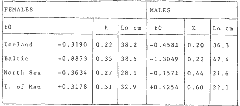

TABLE 6 TEE RATE OF GROWTH WAS CALCULATED USING von BERTALANFFY'S MODEL TO SHOW THE DIFFERENCES ACCORDING TO AREA.

In the Soviet Far Eastern waters Nikol'skii (1961) shows the set of data for Limanda aspera (Pall.) (Table 7).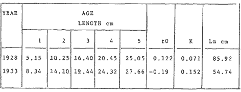

TABLE 7 DATA FOR Limanda aspera IN SOVIET FAR EASTERN.

The parameters of the von Bertalanffy's model calculated were added to this data. In 1928 the fishing exploitation was not intensive, K was low and Lα was high (higher rate of growth). In 1933 the fishing exploitation was intense, then K changed to high and Lα to low, then the rate of growth decreased.

The examples mentioned show that the combination of K and Lα parameters give a good estimate of the rate of growth and they may be useful for fisheries stock assessment.

It well know in fisheries stock assessment that one of the most important findings is to be able to calculate the annual yield curves. So far, length at age has been calculated. It may now be asked, how much does the weight increase when length increases in time?

Figure 6, shows the distribution of individual total weight at age of dab sampled in the area, which was assumed to be representative of the population of dabs around the Isle of Man and might represent an index of Irish Sea.

It was difficult to assess which model would conform to most of the data and be representative. An SPSS package of the computer system was used to give the plot of weight on age of the population sampled (Fig. 6) and the computed straight regression line, by the least square method. Results of the statistics are shown below each figure. The variance (R squared) was 0.5 and 0.47 females and males, respectively. It is clear that the plotted points do not follow this pattern.

Figure 7 shows clearly that the distribution of the points is a curve when the weight on age was plotted as an average, at two monthly intervals. Therefore it was more convenient to use a model describing a curve. Von Bertalanffy's model (as mentioned above) is widely used to conform weight on age (Wt ). Beberton and Holt (1957) used: Wt: Wα (1-e^-k(t-to))³ which is based on Lt: Lα (1-e^-K(t-to)) then in order to obtain Wα he applied the weight-length relationship of the form: Wα = a L³ hence Wα = a Lα ³. where: W = weight of the fish; a constant (the intercept on y axis); L= length of the fish; Wα* = asymptotic weight; Lα* = asymptotic length.

In fisheries biology it is common to relate weight and length as W = aL³ but the exponent 3 does not always occur as expected (Le Cren, 1951). Hence, in order to calculated weight at age, length at age was computed (calculated as described above and converted to weight by applying the actual coefficients of the overall weightlength relationship which has been described (Ortega Salas, 1981a). That gave the following:

Wt= Lt^b; Wt= a (Lα (i-e^k(t-to))^b

where: a = Constant (the intercept on y axis), b Slope (Regression coefficient): Wα = Is calculated as Wα = a Lα^b

The equations may than be written as follows:

FEMALES: Wt = 0.00000495 Lt^3.1998

MALES: Wt = 0.00000566 Lt^3.1091

where: Wt = The whole weight (g) at time (t): Lt Total length (mm) at time (t).

The fitted curves are shown in figure 7: despite the wide range at age and the natural seasonal variation in weight: the theoretical curves showed a good fit to the mean data, and illustrated clearlly that female dab grew bigger than males and reached higher asymptotic weight: 399 g and 1119 females and males respectively.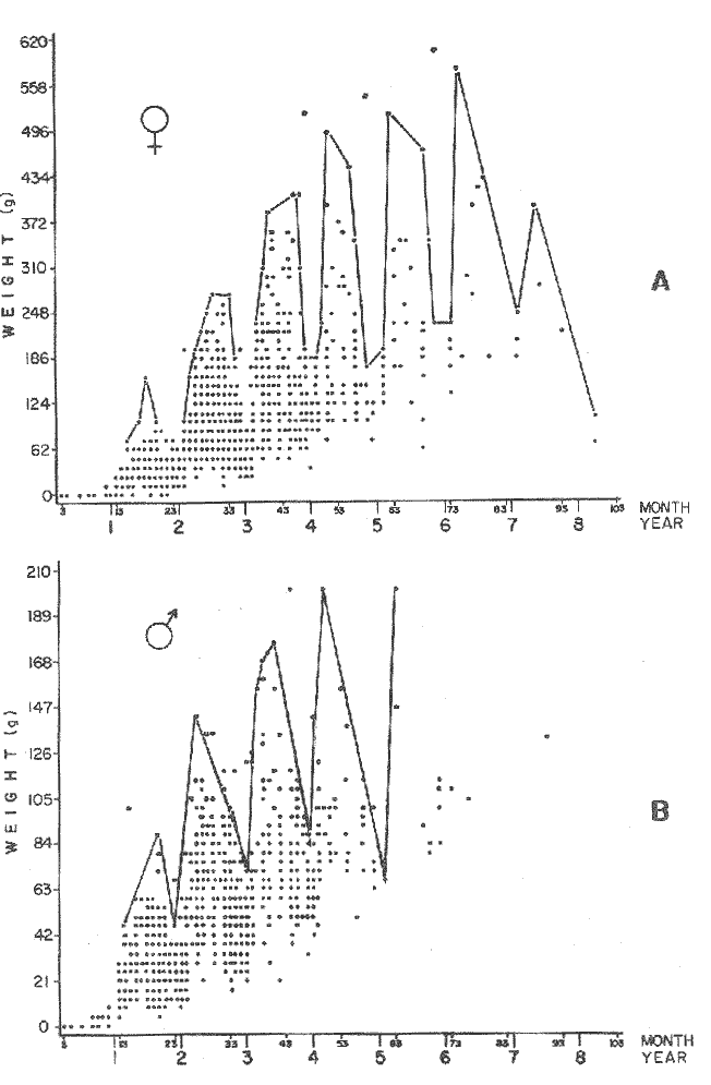

Figure 6. Total weight for age at two monthly intervals. A = females; B = males.

It may be said that length is related in weight in time , and although the fitted curve show that bigger fish weigh more than smaller ones at age, seasonal variation of body weight shows there is a time when bigger fish at age weigh less (winter) than smaller ones (atr age) (summer) (Figs. 6 and 7). Ortega-Salas (1980, 1981a, 1981c) showed there was less food in the stomach in winter than in summer, and that fish in summer tended to grow more than in winter. Growth in weight was more relative, a fish (for a given length) in winter weighed less than a fish in summer.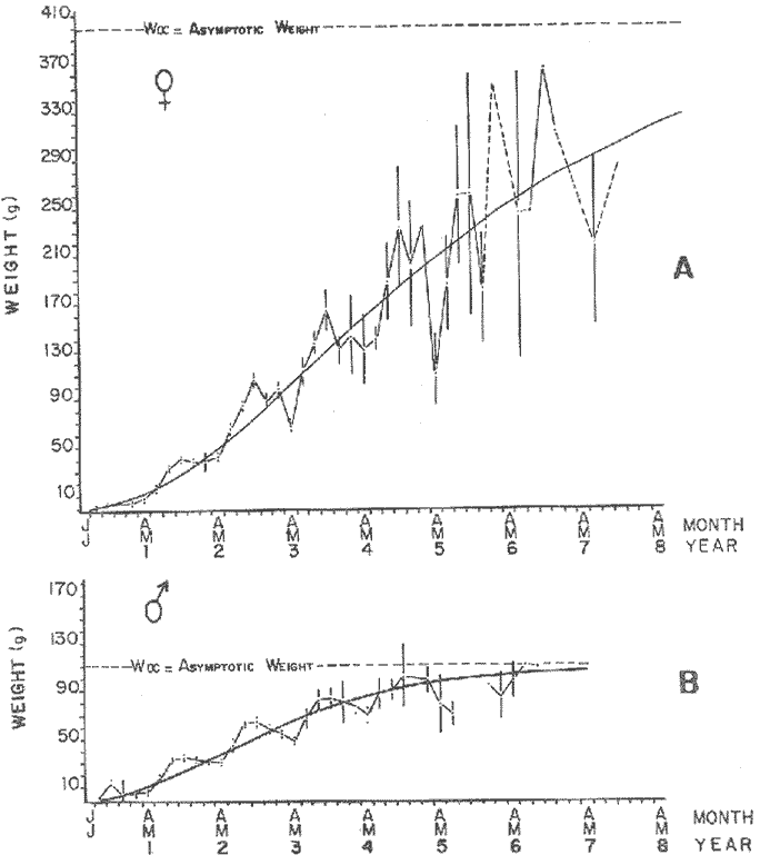

Figure 7. Mean weight for age at two monthly intervals with 0.95 C.I. Theoretical curve fitted. A= females: Wt 3.1398 Lt3.1091.0.00000495 Lt; B = males: Wt = 0.00000566

It is general practice in fisheries to collect data from the main markets where most of the commercial vessels land their catch. Flatfish are usually landed as "gutted" fish but with the gonads included (i.e. Lowestoft and Grimsby landings of flatfish). Therefore, it was decided to obtain similar information for gutted weight fish (guts and gonads removed), as was done for the whole weigh of the fish, in order to calculate the difference. The same procedure (as the whole weight of dab) was used to analyse the gutted weight.

Gutted weight, for age, is shown in figures 8 and 9. The results show a similar pattern to those of the total weight (without the effects of seasonal changes in gonad weight, stomach plus intestine (with contents), and liver weight). Female gonads in winter represent a mean of 16% weight of the gutted weight. In summer, stomach plus intestine together with liver represent an average of 12% weight of the gutted weight (Ortega-Salas 1981a, 1981c).

A von Bertalanffy curve was calculated (as before) using the relationship between gutted weight and length, which has been calculated later (Ortega Salas 1981a) with the following equations

FEMALES: Gutt. wt_t = 0.00000545 L_t^3.10012

MALES: Gutt. wt_t = 0.00000526 L_t^3.1078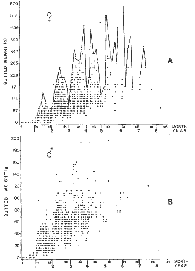

Figure 8. Gutted weight for age at monthly intervals. A = females; B = males.

where: Gutt. wt_t = gutted weight g at time (t):L_t= length mm at time (t).

The theoretical curves in figure g were shown to fit reasonably well. In order to show the mean weight differences between the whole weight and gutted weight for a given length at age a summary was made of the equations, solved as follows: Table 8a, b.

By taking the example of a fish 3.5 years old, the results would be as follows: Table 9.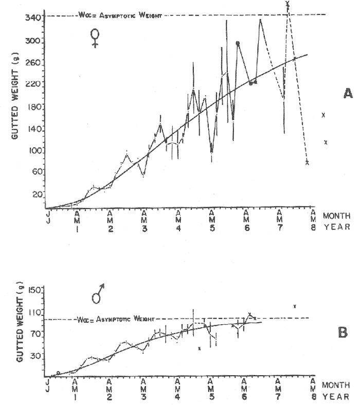

Figure 9. Mean gutted weight for age at two monthly intervals with 0.95 C.I. Theoretical curve fitted. A = females: 3.1001. 3.1076 g.Wt = 0.00000545 Lt ; B = males: g.Wt = 0.00000526 4

For the length calculated in females there was a mean difference of 6% less gutted weight than whole weight, for males it was 4%.

Thus the Table 10, sumarize the difference between the whole weight and the gutted weight (in terms of biomass) according to catch and stock estimated (Ortega-Salas, 1981a, 1981c) for the Irish Sean in 1977.

In biology, by definition, fish species which live longer have a lower natural mortality. In fisheries, Beverton and Holt (1957), Ricker (1975) and others, defined natural mortality (in general terms) as death from other cause other than fishing. In order to be able to assess any fishery, to mantain an optimal yield, it is therefore necessary to calculate the fishing mortality. One way to do so is to estimate natural mortality (which is assumed to be a constant parameter) and relate it to the instantaneous total mortality, to calculate fishing mortality as follows:

z= M + F; z - F= M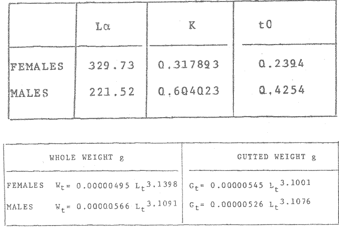

TABLE 8 A) GROWTH PARAMETERS. B) USING THE W-L RELATIONSHIP FOR THE WHOLE AND GUTTED WEIGHT IN TIME.

TABLE 9 APPLICATION OF TABLE 8A AND B IN A FISH 3.5 YEARS OLD.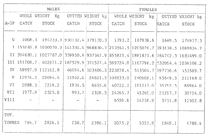

TABLE 10 DIFFERENCES BETWEEN THE WHOLE WEIGHT AND THE GUTTED WEIGHT.

where: z: instantaneous total mortality rate: M: Instantaneous rate of natural mortality: F: Instantaneous rate of fishing mortality. M. estimates are needed for most models presently used in fish population dynamics and Beverton and Holt (1957). Gulland (1969), Ricker (1975) have given several methods to find M.

Weymouth and McMillin (1931) used for the first time Gompertz' equation to calculate the rate of growth of Silique patula (bivalve). The Gompertz' equation was first applied to the graduation rate of human mortality, since the graduation mortality declines through most of the life cycle, as with the growth rate. The rate of declining in growth (K) given by von Bertalanffy gave a good approach to calculate natural mortality (M) as Beverton and Holt (1959) showed for pleuronectides: a relation of M/K ~ 1. Pauly (1980) also used the parameters from von Bertalanffy, together with the mean annual water temperature of the area, in order to calculate M.

Using K as an estimate of M: K may very mainly as a result of fishing effect and to a lesser extent, from one area to another depending on its productivity. So if K varies, M would very in the same proportion, which is reasonable to believe. An under exploited population is considered to have a low K (therefore low M) and high Lα once the population has an intense exploitation. K becomes higher (therefore M higher) and Lα becomes lower, probably, because as older fish are caught, the younger would have more food available, so they become bigger. Nikol'skil (1961) showed exploitation effects on growth for plaice and Limanda aspersa. Older fish (mature) become scarce, so if fishing is greater. M. eventually would be higher since there is constant com petition between species. If mature fish are scarce the result would be less eggs/m² , less larvae/m² and less recruitment, because each stage of life would have the same competition than before the exploitation occurred. The exploited species would be more vulnerable. Eventually ecological equilibrium would be broken by intense fishing of a specific population, the exploited species may never recover; Korringa (1980) mentioned several examples. Fortunately, when a species is exploited there are other species exploited too, which helps to balance the situation within the ecosystem. The problem increases because the modern techniques of fishing are getting very specific to catch single species.

Margalef (1974) mentioned that the growth curve as not strictly a characteristic of the species itself, but of the population of that species and it was as variable as the surviving curve (catch curve). Both had in common that the shape of the fitted points of the curve reflexed the complex interaction of the ecosystem.

The results illustrated that the new program using Holt's method (von Bertalanffy's) gave a good approach to the observed data. The estimated natural mortality (M/K ~ 1) by von Bertalanffy's gave a good approach to the observed data. The estimated natural mortality (M/K ~ 1) by von Bertalanffy's equation was as follows: Females= 0.31; Males= 0.60.

To summarize this study we have the following:

1. The von Bertalanffy's was an appropiate model on growth for dab in the Irish Sea. 2. The environmental conditions affect growth in length and weight of dab in such a way that it is greater in summer than in winter conditions. This also helps to understand the differences in growth from a population of fish which live in an area with better conditions. 3. Theoretical equations relating weight and gutted weight to age showed good fit to the observed mean points, considering the respective weight, and gutted weight-length relationships. 4. There is around 6% difference between this whole weight and gutted weight of the fish. 5. Using the rate of the declining in growth (K) from von Bertalanffy's is considered to give a good estimate figure of natural mortality. 6. The general results of this study on dabs could be applicable to plaice and sole since they are close related species in the wild.

Acknowledgements are due to A. Burd an to C. Bannister for their advise and suggestions. For laboratory facilities to Department of Marine Biology of the University of Liverpool, and MAFF Fisheries Laboratory, Lowestoft. And for the finantial support, Universidad Nacional Autónoma de México: Consejo Nacional de Ciencia y Tecnología; and the British Council.

A) The von Bertalanffy, a) mean length of female dab at each year old, b) mean lengths of male dab at each year old. The a) and b) are shown how to feed the program. Start with "run", type the observed lengths (LT) (a maximum of 100 values), and finish with -1. The output will follow, LT are the calculated values.

B) Gompertz. Feed the program as "A" instructions. The observed values should increaseat each consecutive time.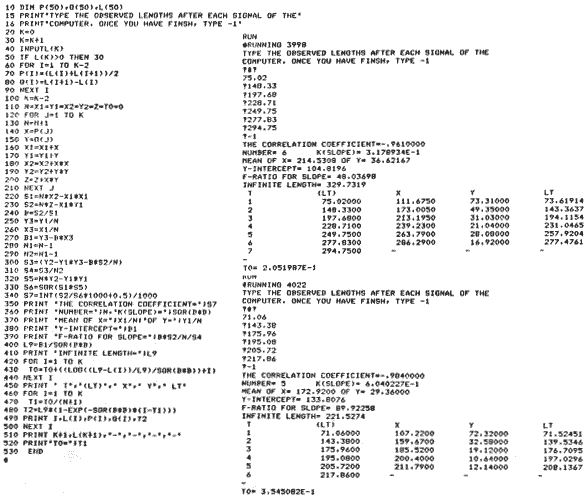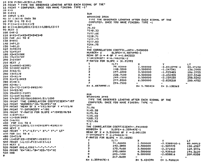

Aviso de Privacidad

Cerrar esta ventana