A USE OF THE CATCH-PER- UNIT EFFORT IN ECOLOGY

Trabajo recibido el 30 de junio de 1980 y aceptado para su publicación el 26 de noviembre de 1980.

RESUMEN

INTRODUCCIÓN

The author (1980) has called generation curves to those showing the relationship between the number of the parent stock and the number of the progeny. If parental and filial generations are censed at the same age a reproduction curve is obtained. If parental stock is censed at the spawning age and the progeny at the recruitment age a recruitment/stock curve is obtained. If the relationship is established between the number of eggs and the resulting recruitment a recruitment/egg curve is obtain ed. Certainly, the latter is not a generation curve because eggs and recruits belong to the same generation; more properly, it is a survival curve. However, during the egg-recruitment span events take place that characterize the shape of the other two curves; so it is necessary to take this into account for the general study of the generation curves.

For a determined species recruitment/stock an reproduction curves follow the same model, which is that of the recruitment/egg curve, but the parameters of the three curves are different and also their properties respecting the fishing (Larrañeta, 1980).

In this paper a use of the catch-per-unit effort is explored to discriminate ecological changes, based on previous studies of the generation curves.

Larrañeta (1979) has examined the biological meaning of the parameters of the Beverton-Holt and Ricker models applied to the reproduction curves; that is, when parental (P) and filial (R) stocks are measured at the same age. Above-mentioned are,

and

R= APe -BP (Ricker, 1958)

Parameters A and 1/β mean the number of eggs laid per fish that survival until the age of replacement in the absence of compensatory mortality, and they depende on physiological and constitutional (genetic) factors and on the ecological niche. On the other hand, Parameter B is related to the compensatory mortality which depends on factors such as the initial density of food organisms, replacement age, and fecundity Larrañeta, 1979).

As a general assertion, marine fish populations have generation curves belonging to the Ricker model, that is, dome-shaped curves, more or less domed, sometímes being merely an increasing curve until they arrive at an equilibriura point. On the contrary, the Beverton-Holt model always yield an asymtotic curve, the asymptotic level being 1/α, and it seems to be more appropiate for flatfish species. From an analysis of Larrañeta (1979) it is deduced that, actually, the Beverton and Holt model will be proper of those species with a very strong territorial competition at the fixation or recruitment, the limited area being the principal factor determinig the asymptotic: number l/α. It is also posible to produce an asymptotic curve throughout a very severe food limitation, in such a way that inter-larval competition is the principal factor of the compensatory mortality.

As the Ricker model seems to be the more general case the discussion will be limited to this model. The mathematical expression of the Ricker model (1958) was given by Beverton and Holt (1957) but they considered it as a secondary case in the general stock-recruitment problems; afterwards, Ricker used it for the conceptual model which he has been studying since his paper written in 1954.

Moving from reproduction curves to the recruitment/egg and recruitment /stock curves, the numerical value of Parameter A is not the same in the three curves, but the biological meaning remains the same; that is, Parameter A is a representation of survival in relationship with the abiotic environment, the ecological niche and the genotype. A large-scale change in any of these three factors will modify Parameter A. The environment is considered in itself to be all the factors that determine physiological rates, specially as refering to temperature, salinity and light, but also to pressure, turbulence, pollution, etc., as direct or indirect factors of the vital activity of a determined species.

On the other hand, Parameter B, being associated to the initial food supply, will also be associated with the primary productivity, the area size with suitable larval food, the patchiness of the food and other factors determining the food availability, which, in turn, are associated with meteorologic and hydrog raphic phenomena. A storm can disperse the larval food and cause failure of an important fraction of the recruitment, but in generation dynamics variations of Parameter B are only produced by large-scale time changes.

Summarizing, direct and indirect factors which can produce changes in Parameters A and B can be listed as follows,

Parameter A

Abiotic environmental factors (temperature, salinity, light, pollutans, etc.).

Ecological niche (Relative importance of the principal predator, competitor and prey species).

Genotype (physiological and constitutional features).

Parameter B

Average fecundity of the stock.

Initial larval food suply.

Patchiness of the food area.

Large-scale hydrographic events modifying the size and/or the food density of the nursery area (e.g. stream changes).

According to the Ricker model recruitment (R) is related to stock (S) as follows

R= ASe -BS (1)

The total spawning stock is S = σS i, where S i is the number at age i of the mature individuals. To simplify this, it can be supposed that the spawning stock consists only of one agegroup. Then

S= Re -Z

where Z is the total mortality between the recruitment age and the spawning age.

In a steady state the stock (S') and the recruitment (R') are constant, so substituting in (1) S' for R',

R' = AR'e- ZeBS'

or

1nR' = 1nA + 1nR' - Z - BS'

and eliminatino, 1nR',

BS' = 1n (Ae -Z)

S' = 1/B 1n (ae-Z)

On the other hand, all fishes recruited will die either by natural causes (M) or by fishing (F). In the total life span the fishing rate is F/Z, and the equilibrium catch of an annual class is:

C' = R' (F/Z)

and the equilibrium catch per unit effort will be

U' ~ R' / Z

Therefore, if parameters A and B and total mortality are given, parental population in equilibrium (S') is obstained by (2), recruitment (R') is obtained by (1) and an index of the catch per unit effort (U') by (3).

At the top of Figure 1 three recruitment/ sotck curves are shown, with the following parameters: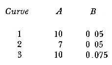

Using expressiones (1), (2) and (3) three catch-per-unit effort curves are obtained, as is shown at the bottom of figure 1.

In this case, the shape of the catch-per-unireffort curves has no special importance, but it seems interesting to realise that taking Curve 1 as the initial curve, departure of Curves 2 and 3 has different features in each case. In fact, when Parameter A varies it seems that levels at F = 0 and U = 0 are different but diverge, on the right, as is shown schematically in figure 2, side A. Curve 2 hasta a lower position than Curve 1 when Parameter A decreases.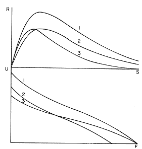

Fig. 1. At the top, three recruitmentl /stock curves; curves 1 and 2 with the same compensatory mortality, and curves 1 and 3 with the same density-independent mortality. At the bottom, catch-per-unit-fishing-mortality curves derived from the previous recruitmentl /stock curves.

On the other hand, Curves 1 and 3 have a different level at F = 0 but the same point at U = 0, converging on the right, as is shown schematically in figure 2, side B. Curve 3 has a lower position as Parameter B increases.

Therefore, when plotting U against f , wheref is the fishing effort -F = fq, whereqis the catchability coefficient - if annual points lie within two historical series, with regression lines diverging or converging at the right, it will be a sign of change in factors associated to Parameter A or to Parameter B of the recruitment /stock curve, respectively.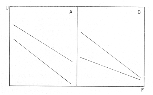

Fig. 2. Schematic variations of the c.p.u.e. trend when changes in Parameter A or B of the Ricker model occur.

One other interesting point is that if from the U/F curves the corresponding Y/F curves are derived, because

Y = UF

it appears then that Curves 2 and 3 have a lower maximum sustainable yield (MSY) than Curve 1, but Curves 1 and 3 have the MSY at the same fishing mortality (F MSY) and Curve 2 at a smaller one (Fig. 3). This feature can be very important for management purposes.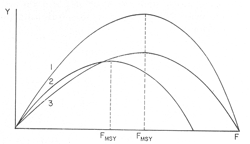

Fig. 3. Yield curves derived from curves of Figure 1.

Recently, Vázquez and Larrañeta (1980) have studied the dynamics of the cod(Gadus morhua) stock in Divisions 3NO (Southern part of the Grand Bank of Newfoundland) of the NA FO Area, and they have found that points of the catch-per-unit effort lie within two historical series, as is shown in figure 4 by regression lines. The series 1954-1957 and 1963-1972 belong to the first regression line, and the series 1958-1962 and 1973-1977 belong to the second one. It could be argued that these two regression lines might be a subjective impression, but a very similar phenomenon is found by taking the data of Gavaris (1980) on cat-per-unit effort in the cod fishery of Div. 3M of the NAFO Area, and plotting them against effort, where two regression lines, fitted by us, also-appear; the first one for the period 1960-1972 and the second one for the period 1973-1979 (Fig. 5). In both 3M and 3NO fisheries a leap from regression 1 to regression 2 takes place at the same time, that is, between the years 1972 and 1973.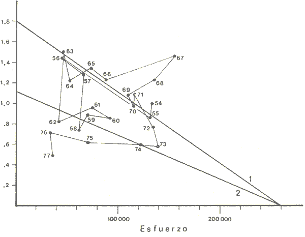

Fig. 4. Catch-per-unit-effort regressions in the NAFO 3NO cod fishery (Vázquez and Larrañeta, 1980).

If the regression lines meet at the right side, just on the effort axis, it means, according to the previous discussion, that a change in Parameter B of the recruitment/stock curve can be suspected. If so, some of the causes listed as related to Parameter B can be taken ínto consideration, such as larval food availability, caused by changes in the general marine current system, which would be the most logical event for us.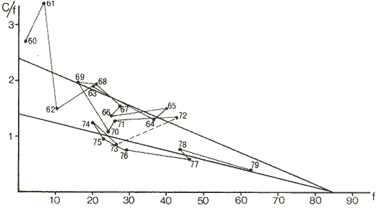

Fig. 5. Catch-per-unit-effort regressions in the NAFO 3M cod fishery according to data from Gavaris (1980).

A very similar example is found for the sardine (Sardina pilchardus) of Castellon (Spanish Mediterranean coast) by Larrañeta (1981). In this case the regression lines meet at the right also, but not upon the effort axis but somewhat higher (Fig. 6). However, two historical series of points very clearly seem to belong to two regression lines, the first one for the 1956-1964 period and the second one for the 1965-1969 period. Larrañeta (1981) has found that between these two periods some changes have taken place as, for example, a decrease of the sardine density followed by an increase of the anchovy (Engraulis encrasicholus) catches. At the same time, oceanographic events were detected in the way of a change of the current pattern of the area. That is, there was not a direct competition between the anchovy and the sardine populations but a change of the environment favoring the anchovy population and restrincting the sardine population, because plankton productivity was more suitable to the anchovy population during the second period. All these features are related to a change of Parameter B by increasing the compensatory mortality of the sardine.

Larrañeta (1981) has estimated a new recruitment/egg curve for the second period of the Castellon sardine population by increasing Parameter B, and deduced the consequences as far as the yield is concerned, which are in accordance with the observed catches.

Maigret (1979) gives an interesting example of the trap fishery stock of the rose lobster(Palinurus mauritanicus) in the Mauritanian coast. A change occurred in this fishery between 1962 and 1969 because a very heavy trawling fishery was developed, which has reduced the distribution area of the population to the canyons where trawling fishery is not possible. Maigret found two apparent equilibrium lines between catch-perunit effort and effort (Fig. 7).

In this rose lobster fishery the regression lines diverge to the right side, the same as when a change in Parameter A was tested. Maigret's conclusions on the Schaefer curves of Y/f for the two fishing situations are similar to our conclusions when Parameter A is reduced (Curves 2, in Fig. 1 and 2). But if fishing intensity instead of fishing effort is taken into consideration, the picture appears as in Figure 8, as taken from Figure 4 of Maigret's paper. In figure 8 the 1967-1975 series appears above the 1958-66 series, the reverse than in figure 7. The two series of figure 8 could yield regressions which would have the same U level when fishing intensity is very close to zero. This means that the density in the canyons is the same than that in the continental shelf when there is no fishing. If so, both regerssions of figure 7 must have also the same U level when fishing effort is very close to zero.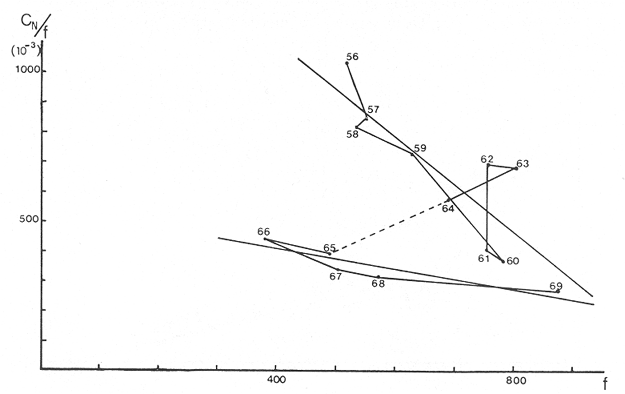

Fig. 6. Catch-per-unit-effort regressions in the Castellon sardine fishery (Larrañeta, 1981).

We think that in figure 7 the 1968-1975 regression slope is greater than that of the 1958-1963 regression because the same effort is applied to a smaller area and, therefore, with the same effort the físhing mortality was greater in 1968-1975 than in 1958-1963. But if this effect is corrected by relating U with the fishing intensity (Fig. 8) then the 1958-1966 series has a greater slope than that of the 1967-75 series. This is so because the fishing effort on the continental shelf was underestimated due to the fact that the trawling fishing effort was not taken into account, so the great slope of the 1958-1966 series in Figure 8 would be an artifact.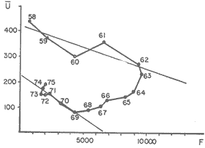

Fig. 7. Catch-per-unit-effort regressions in the Mauritanian rose lobster fishery (Maigret, 1979).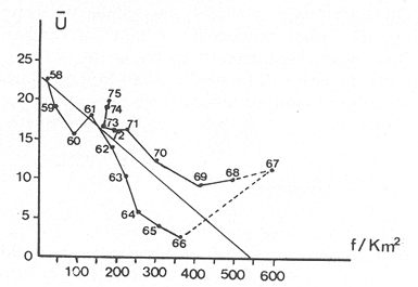

Fig. 8. Catch-per-unit fishing intensity in the Mauritanian rose lobster fishery (Maigret, 1979).

According to the above considerations, it seems that regressions of figure 7 would not represent a real example of variations in Parameters A; so, it is necessary to be careful when analyzing fisheries throughout historical series of catch-per-unit effort, as it was proposed here. The difference between a real case of a change in Parameter A and that of the rose lobster fishery is that in the former both regressions must show a different density when there is not any fishing effort, and in the rose lobster fishery it seems that both regressions have the same initial U level, as it apears in figure 8.

In the literature available there appears to be some confusion in the nature of what we call generation curves, because the three classes of curves shown here have different properties respecting the fishing. For example, fishing reduces Parameter A of the reproduction curve (Larrañeta, 1979), the greater the fishing effort the greater the reduction of Parameter A, until the populations is extinguished when A arrives at 1. In some circumstances recruitment/egg and recruitment/stock curves can also be modified by fishing, and these effects have been analyzed in another paper (Larrañeta, 1980) but, as a first approach, we can suppose that they are not modified by fishing. On this assumption the present study has been developed, because of some effect were produced it would not esentially change the conclusions.

The relationship between the recruitment/stock curve and the catch-per-unit effort has been developed taking numbers but weight of chatches into account. However, c.p.u.e. of current studies is given as cacht-weight, but we think that this does not change our conclusions esentially. For example, when Parameter B varies, U and Y become zero at the same fishing effort level and, obviously, it will be the same to take either number or weights ot catches. Also, when Parameter B increases the MSY of the Y/f curve will be smaller than formerly but, according to our estimations in a previous paper (Larrañeta, 1981: Cuadros 16-21) if Parameter B increases, F MSY also increases, the greater the natural mortality, the greater the FSMY increase will be. This means that with a greater Parameter B, although a lower MSY is produced, danger of overfishing is not greater but, on the contrary, rather reduced.

In conclusion, we thing that it is interesting to take into account historical variations of the catch-per-unit effort, as is shown in this paper, to analyze ecological changes in the fishery resources, although these variations must not be taken, of course, automatically, but through a critical viewpoint, as was done in the Mauritanian lobster fishery case.

I am indebted to Antonio Vázquez for his useful comments about generation curves and catch-per-unit effort, and to Paty Briones for her review and comments on this paper.

Aviso de Privacidad

Cerrar esta ventana